
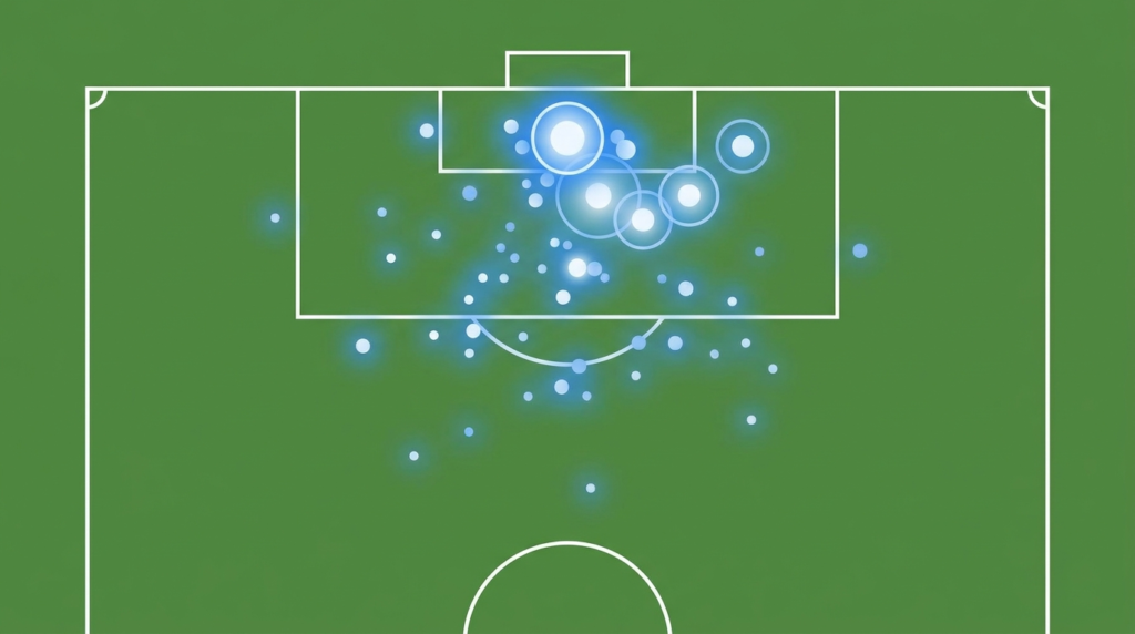
Expected Goals (xG) has become the most talked-about metric in modern football analysis. If you follow football betting, fantasy football, or tactical discussion, you have almost certainly encountered xG. But what exactly is it, how is it calculated, and more importantly, how can you use it to make smarter betting decisions?
In this guide, we explain expected goals from the ground up, show you where to find reliable xG data, and demonstrate how to apply it to your football betting strategy. Whether you are a complete beginner or someone who has heard the term but never fully understood it, this guide will give you everything you need to start using xG effectively.
The rise of xG has transformed how we understand football. Before advanced metrics became widely available, fans and pundits judged teams almost entirely by results. A team that won 2-0 was playing well; a team that lost 1-0 was playing poorly. xG revealed that this surface-level analysis was often wrong. A team could win 2-0 while creating almost nothing of quality, and a team could lose 1-0 while dominating the chance creation. Understanding this distinction is the first step toward using xG for betting advantage.
For bettors, xG is particularly valuable because it cuts through the noise of individual match results and reveals the underlying quality of team performance. While actual goals are influenced by luck, finishing quality, and random events, xG provides a more stable and predictive measure of how well a team is playing. This makes it an invaluable tool for identifying value in the betting market.
What Is Expected Goals (xG)?
Expected Goals is a statistical metric that measures the quality of a scoring chance. Every shot in a football match is assigned an xG value between 0 and 1, representing the probability that the shot will result in a goal. A penalty kick typically has an xG of around 0.76 (76% chance of scoring), while a shot from 35 yards out might have an xG of just 0.02 (2% chance).
The key insight is that xG tells you whether a team is creating good chances or just getting lucky. A team that wins 2-0 but only generated 0.4 xG was fortunate. A team that loses 1-0 but created 2.3 xG was unlucky and likely to improve in future matches.
Think of xG as a way to measure what should have happened rather than what did happen. If a team takes ten shots from inside the box, each with an xG of 0.10, their total xG for the match is 1.0. This means that, on average, we would expect them to score one goal from those chances. If they actually scored three goals, they overperformed their xG by 2.0 goals, suggesting they were either exceptionally clinical or simply lucky.
The concept of expected goals is not unique to football. Similar metrics exist in basketball (expected points per shot), hockey (expected goals based on shot location and type), and even baseball (expected batting average based on exit velocity and launch angle). The underlying principle is the same: use historical data to estimate the probability of success for each attempt, then sum those probabilities to get an expected total.
What makes xG particularly powerful in football is that goals are relatively rare events. In a typical match, there might be only 2-3 goals scored from 20-30 shots. This means that individual goals carry enormous weight in the result, and a single lucky deflection or world-class save can completely change the outcome. xG smooths out this randomness by looking at the quality of all chances created, not just the ones that resulted in goals.
It is important to understand that xG is not a perfect measure. It does not account for the skill of the shooter, the quality of the goalkeeper, or the tactical context of the shot. A shot taken by Erling Haaland from a given position is more likely to result in a goal than the same shot taken by a centre-back. However, xG models typically do not differentiate between shooters, which means they treat all shots from the same position as equally likely to score. This limitation is worth keeping in mind when using xG for analysis.
How Is xG Calculated?
xG models analyse thousands of historical shots to determine the likelihood of scoring from any given situation. The main factors include shot location, type of assist, body part used, defensive pressure, game situation, and shot type. Each of these factors contributes to the final xG value assigned to a shot.
Different data providers (Opta, StatsBomb, FBref) use slightly different models, but they all follow the same fundamental principle: compare each shot to thousands of similar historical shots to estimate its scoring probability. The more data a provider has, the more granular and accurate their model can be.
Shot location is by far the most important factor in xG calculation. Shots taken from closer to the goal and from central positions have higher xG values than shots from distance or wide angles. A shot from the six-yard box might have an xG of 0.50 or higher, while a shot from 25 yards out might have an xG of just 0.03. This reflects the simple reality that shots from closer range are more likely to result in goals.
The type of assist also plays a significant role. A shot following a through ball or a cutback from the byline typically has higher xG than a shot following a long cross or a loose ball. This is because certain types of assists create better scoring opportunities. A through ball that splits the defence and puts a striker one-on-one with the goalkeeper is a high-quality chance, while a hopeful cross from 30 yards out is not.
Body part matters too. Headers generally have lower xG than foot shots from the same position because they are harder to control and direct accurately. However, a header from close range following a well-delivered cross can still have a high xG value. Some advanced models also factor in whether the shot was taken with the player’s preferred foot, as this can affect accuracy and power.
Defensive pressure is increasingly incorporated into modern xG models. A shot taken with a defender closing down rapidly has lower xG than the same shot taken with time and space. Some models use tracking data to measure the distance and speed of the nearest defender, while others use simpler proxies like the number of defenders between the shooter and the goal. The more sophisticated the model, the better it can account for these contextual factors.
Game situation also influences xG. Shots taken in open play, from set pieces, and on counter-attacks have different scoring rates even from the same location. A penalty kick has a fixed xG of around 0.76 regardless of who takes it, because the historical data shows that approximately 76% of penalties result in goals. Free kicks and corners have their own xG values based on historical conversion rates from similar situations.
Why xG Matters More Than Actual Goals
Actual goals are noisy. A single match can be decided by a deflection, a referee decision, or a moment of individual brilliance that no model could predict. Over a small sample, luck plays a huge role. xG strips away that noise and shows you the underlying performance.
Consider these real-world examples from recent Premier League seasons. Team A scored 68 goals but only generated 52 xG, meaning they overperformed by 16 goals. Team B scored 41 goals but generated 58 xG, meaning they underperformed by 17 goals. In the following season, Team A typically regresses toward their xG (scoring fewer goals), while Team B typically improves (scoring more). This regression to the mean is one of the most reliable patterns in football analytics.
This regression phenomenon is crucial for bettors to understand. When a team has been overperforming their xG for an extended period, the market may still price them as a strong team based on their actual results. This creates value opportunities on the other side. Conversely, a team that has been underperforming their xG may be undervalued by the market, presenting betting opportunities on them to improve.
The key is to look at xG over a meaningful sample size. One match tells you very little. Five matches give you a rough indication. Ten or more matches provide a reliable picture of a team’s underlying performance. Professional analysts typically look at xG over the last 10-20 matches to assess current form, while also considering the full season xG to understand longer-term trends.
It is also worth noting that xG can reveal tactical changes before they show up in the results. If a team has appointed a new manager and their xG has increased significantly over the last five matches, this suggests the new tactics are working even if the results have not yet improved. This forward-looking aspect of xG makes it particularly valuable for in-season betting.
However, xG should not be used in isolation. The best analysts combine xG with other metrics like expected goals against (xGA), expected points (xPTS), and possession-based metrics to build a complete picture of team performance. xG tells you about attacking quality, but you also need to understand defensive quality, set-piece effectiveness, and other factors to make fully informed betting decisions.
How to Use xG for Football Betting
xG can be applied to football betting in several powerful ways. The key is to use xG data to identify discrepancies between a team’s underlying performance and the market’s perception of that performance. When you find such discrepancies, you have identified a potential value bet.
The most effective xG-based betting strategies focus on medium to long-term trends rather than individual matches. While xG can inform single-match betting decisions, its real power lies in identifying teams that are systematically mispriced by the market due to overperformance or underperformance of their underlying metrics.
Let us explore the main ways xG can be used for betting advantage.
1. Identify Teams Due for Regression
When a team has been winning but their xG is significantly lower than their actual goals scored, they are likely overperforming and due for a downturn. Conversely, a team losing despite high xG is creating good chances and may be undervalued by the market.
This is particularly useful for betting on upcoming fixtures. If a team has underperformed their xG over the last 5-10 games, the market may still price them as poor form, creating value on the other side. The key is to quantify the underperformance. A team that has scored 8 goals from 15 xG over their last 10 matches is underperforming by 0.7 goals per game, which is a significant discrepancy that is likely to correct over time.
Regression betting works best when combined with other factors. A team that is underperforming their xG AND has a favourable upcoming fixture list presents a stronger betting opportunity than a team that is underperforming but faces a run of difficult opponents. Always consider the context when using xG for regression betting.
It is also important to consider why a team is overperforming or underperforming. Sometimes there are legitimate reasons for sustained deviation from xG. A team with an elite finisher like Harry Kane or Mohamed Salah may consistently overperform their xG because their striker converts chances at a higher rate than average. Conversely, a team with poor finishing may consistently underperform. Understanding these contextual factors helps you distinguish between temporary variance and genuine skill differences.
2. Evaluate Player Performance
xG helps you assess whether a striker is genuinely clinical or just riding a hot streak. A forward scoring 20 goals from 12 xG is finishing at an elite rate, but this is rarely sustainable. Conversely, a striker with 8 goals from 14 xG is finishing poorly but creating excellent chances, suggesting improvement is likely.
For prop bets like “anytime goalscorer,” xG per 90 minutes is one of the most reliable predictors of future scoring. A striker who averages 0.50 xG per 90 minutes is creating half a goal’s worth of chances every game, which translates to roughly one goal every two games. This is a much more stable predictor than actual goals scored, which can be heavily influenced by short-term variance.
Player xG data is also useful for identifying undervalued players in the transfer market. A striker who is underperforming their xG at their current club may be a good signing for a team that needs goals, because their underlying chance creation is strong even if their finishing has been poor. This type of analysis is used by professional scouts and data analysts across the football industry.
When evaluating players, it is important to consider the quality of chances they are getting, not just the volume. A striker who takes 5 shots per game from low-xG positions may have a lower total xG than a striker who takes 2 shots per game from high-xG positions. The latter striker is likely to be more efficient and may be a better betting proposition for goalscorer markets.
3. Assess Team Matchups
Compare the xG created by one team against the xG conceded by their opponent. If Team A creates 1.8 xG per game and Team B concedes 1.6 xG per game, you can expect a high-scoring affair. This is far more predictive than looking at goals scored and conceded, which are distorted by luck and finishing variance.
This matchup analysis is particularly powerful for over/under total goals markets. If both teams have high xG created and high xG conceded, the over is likely to be good value. If both teams have low xG created and low xG conceded, the under may present value. The key is to compare the attacking xG of one team with the defensive xGA of the other to estimate the likely total xG for the match.
For example, if Team A creates 1.8 xG per game and Team B concedes 1.4 xG per game, you might estimate that Team A will create around 1.6 xG in this matchup (somewhere between their average and their opponent’s defensive average). Do the same calculation for Team B, and you have an estimated total xG for the match. Compare this to the over/under line offered by bookmakers to identify value.
Home and away splits are important in matchup analysis. Many teams perform significantly differently at home versus away, both in terms of xG created and xG conceded. Always use home/away specific xG data when available, rather than overall season averages, for more accurate matchup assessments.
4. In-Play Betting Opportunities
During live matches, xG can reveal which team is dominating chances even if the scoreline suggests otherwise. If the underdog is 1-0 up but has only 0.2 xG while the favourite has 1.5 xG, the favourite is likely to equalise. This creates live betting opportunities that the casual punter misses.
Live xG data is available from several providers and can be a powerful tool for in-play betting. The key is to act quickly when you identify a discrepancy between the scoreline and the underlying xG. If a team is losing but has created significantly more xG than their opponent, the live odds on them to equalise or win may offer excellent value.
However, live xG betting requires quick decision-making and a good understanding of how xG accumulates over the course of a match. Early xG dominance does not always translate to late goals, especially if the leading team is defending deep and absorbing pressure. Context matters: a team dominating xG in the first 20 minutes against a team that is happy to sit back and counter may not be as dominant as the raw xG numbers suggest.
It is also worth noting that live xG data can be less reliable than pre-match xG data because the sample size within a single match is small. A single high-xG chance can dramatically shift the live xG totals, so it is important to look at the number and quality of chances, not just the total xG figure.
Where to Find xG Data
Several free and paid sources provide xG data for football matches. The quality and depth of data varies significantly between providers, so it is worth exploring multiple sources to find the one that best suits your needs.
For most bettors, free sources provide more than enough data to start using xG effectively. Premium sources offer more granular data and additional metrics, but the core xG figures are generally consistent across providers.
Here are the main sources of xG data:
FBref.com: Free xG data for major leagues, powered by StatsBomb. FBref is one of the best free sources of xG data, offering detailed statistics for the top European leagues, MLS, and several other competitions. The data includes xG for and against, xG per shot, and player-level xG figures. FBref also provides historical data going back several seasons, which is invaluable for trend analysis.
Understat.com: Detailed xG maps and shot-by-shot breakdowns for top European leagues. Understat is particularly useful because it provides visual xG maps that show exactly where each shot was taken and its xG value. This visual representation helps you understand not just how many chances a team created, but where those chances came from and how dangerous they were.
WhoScored.com: xG data alongside other advanced statistics. WhoScored provides xG data as part of their comprehensive match statistics, along with player ratings, heat maps, and other analytical tools. While their xG model may differ slightly from StatsBomb or Opta, it is still a useful source for general analysis.
Opta Analyst: Professional-grade xG analysis and articles. Opta is the gold standard for football data, and their Analyst platform provides in-depth xG analysis along with other advanced metrics. While some content is behind a paywall, they also publish free articles that demonstrate how to use xG for match analysis and betting insights.
For serious bettors, building your own xG model or subscribing to a premium data service can provide an edge over the market. However, this requires significant technical expertise and access to detailed shot-level data, which is expensive. Most bettors will find that free sources like FBref and Understat provide more than enough data to implement effective xG-based betting strategies.
Limitations of xG
While xG is a powerful tool, it is not perfect. Understanding its limitations helps you use it more effectively and avoid common pitfalls that can lead to poor betting decisions.
It does not account for goalkeeper quality: A shot with 0.3 xG against a world-class keeper has a lower actual probability than the same shot against a weak keeper. This means that xG can overestimate the likelihood of goals against elite goalkeepers and underestimate it against poor ones. When analysing matches involving teams with exceptional or terrible goalkeepers, adjust your xG expectations accordingly.
It does not capture defensive positioning: Two shots from the same location may have very different difficulty levels depending on how defenders are positioned. A shot with a clear path to goal is more likely to score than a shot that needs to navigate through a wall of defenders. Some advanced xG models attempt to account for this using tracking data, but most publicly available xG figures do not include this level of detail.
It is backward-looking: xG models are built on historical data and may not capture tactical innovations or changes in playing style. If a team has adopted a new tactical approach that creates different types of chances than those in the historical dataset, the xG model may not accurately reflect the quality of those chances. This is particularly relevant when analysing teams that have recently changed managers or playing styles.
Sample size matters: xG becomes reliable over 10+ games. Drawing conclusions from a single match is risky. A team can easily overperform or underperform their xG in any given match due to variance. Always look at xG trends over multiple matches before making betting decisions based on xG data.
It does not account for game state: A team that is 2-0 up may stop creating chances because they are happy to defend their lead. Their xG for the match may be low, but this does not mean they played poorly — it means they changed their approach based on the scoreline. Understanding game state context is essential for accurate xG interpretation.
Combining xG with Other Metrics
The best analysts combine xG with complementary metrics to build a more complete picture of team performance. Using multiple metrics together gives you a more robust and reliable assessment than any single statistic alone.
xGA (Expected Goals Against): Measures the quality of chances a team concedes. While xG tells you about attacking quality, xGA tells you about defensive quality. A team with high xG and low xGA is creating good chances while preventing the opposition from doing the same — this is the profile of a strong team. Combining xG and xGA gives you expected goal difference (xGD), which is one of the most predictive metrics in football.
xPTS (Expected Points): Estimates how many points a team should have based on xG and xGA. This metric simulates match outcomes based on the underlying xG data and calculates how many points a team would be expected to earn. Comparing actual points to xPTS reveals whether a team is overperforming or underperforming relative to their underlying performance.
PPDA (Passes Per Defensive Action): Measures pressing intensity. A low PPDA means a team presses aggressively, forcing opponents to play more passes before making a defensive action. This metric helps you understand a team’s defensive approach and can be combined with xGA to assess whether a team’s defensive record is sustainable.
Field tilt: Shows which team spends more time in the attacking third. Field tilt is calculated as the proportion of final third passes made by one team compared to the total final third passes by both teams. A high field tilt indicates territorial dominance, which often correlates with xG dominance but can also reveal teams that dominate possession without creating high-quality chances.
By combining these metrics, you can build a multi-dimensional assessment of team performance that is far more reliable than any single metric. For example, a team with high xG, low xGA, low PPDA, and high field tilt is dominating in every aspect of the game and is likely to be undervalued by a market that focuses only on recent results.
Practical xG Betting Strategy
Here is a simple framework you can apply immediately to start using xG for football betting. This strategy focuses on identifying value opportunities based on xG trends and market mispricing.
Step 1: Check the last 5-10 games for both teams. Compare actual goals to xG for each. Calculate the difference between actual goals and xG for both teams over this period. A difference of more than 0.3 goals per game in either direction is significant and worth investigating further.
Step 2: Identify any significant overperformance or underperformance. Teams that are overperforming by more than 0.3 xG per game are candidates to fade (bet against). Teams that are underperforming by more than 0.3 xG per game are candidates to back (bet on). The larger the discrepancy, the stronger the signal.
Step 3: Compare xG created vs xG conceded for the matchup. If one team creates significantly more than the other concedes, that is your edge. Calculate the expected total xG for the match by averaging each team’s attacking xG with their opponent’s defensive xGA. Compare this to the over/under line to identify value in total goals markets.
Step 4: Check the market odds. If your xG analysis suggests a different outcome than the odds imply, you have found a value bet. Convert the odds to implied probability and compare with your xG-based assessment. If your assessed probability is higher than the implied probability, you have identified value.
Step 5: Track your results. Keep a record of your xG-based bets and review them monthly to refine your approach. Include the xG data that informed each bet, the odds taken, and the outcome. Over time, this data will help you identify which types of xG-based bets are most profitable and which need adjustment.
Conclusion
Expected Goals is not a crystal ball, but it is the closest thing football analytics has to one. By focusing on the quality of chances rather than the randomness of actual goals, xG gives you a clearer picture of team performance and future outcomes.
The bettors who consistently profit are those who combine xG analysis with disciplined bankroll management and an understanding of market inefficiencies. Start by tracking xG for your favourite leagues, compare it to the odds, and look for discrepancies. Over time, this approach will give you a significant edge over punters who rely on gut feeling and surface-level statistics.
Remember that xG is a tool, not a complete solution. The best bettors use xG as part of a broader analytical framework that includes tactical analysis, team news, motivation factors, and market dynamics. xG gives you a quantitative foundation for your analysis, but the qualitative context is equally important. Combine the numbers with your football knowledge, and you will be well-equipped to find value in the betting market.